Fraud Detection
November 17, 2017
For details and code, please visit my Jupyter Notebook.
Project is still in progress!
Credit Card Fraud Detection
Objective
The aim of this project is to experiment different approaches to dealing with fraud detection and to understand the pros and cons of each. Recall score is our priority because the consequences are more dire if we misclassify a true fraud case as non-fraud. Precision score is important as well, but its impact is less serious than recall score in terms of credit card fraud. Choosing or balancing between both of these scores will depend on the context of the problem; e.g. real world business needs (whether or not we require a maximum score for either metric, or a balance of both).
Data
This is a popular dataset from Kaggle.
Out of 284,807 data rows, only 492 are fraudulent transactions. That's extremely imbalanced at 0.173%!
The dataset contains transactions made by credit cards in September 2013 by european cardholders, over a period of two days. It contains only numerical input variables which are the result of a PCA transformation. Unfortunately, due to confidentiality issues, the original features and more background information cannot be provided. Features V1, V2, ... V28 are the principal components obtained with PCA, the only features which have not been transformed with PCA are 'Time' and 'Amount'.
'Time' contains the seconds elapsed between each transaction and the first transaction in the dataset.
'Amount' is the transaction Amount, this feature can be used for example-dependent cost-senstive learning.
'Class' is the response variable and it takes value 1 in case of fraud and 0 otherwise.
Overview
The data has PCA features V1 ~ V28, Time, Amount, and Class. For our initial analyses, we will be putting aside the Time and Amount and focus on testing models on just the 28 features.
- Exploratory Data Analysis
- Manual Under-Sampling modelled with Logistic Regression
- Sampling methods with IMBLearn package
- Logistic Regression
- Random Forests
- XGBoost
- Ensemble Sampling
- Autoencoder Neural Net
- Cost Sensitive Learning
- Clustering
- Isolation Forest
- One-Class Support Vector Machine (SVM)
- White Magic / Dark Art Ensemble
Exploratory Data Analysis
First, we visualized correlations using seaborn's heatmap. Since the V features are obtained through Principal Components Analysis, we would not expect them to be correlated. Next, we took a look at 'Amount' vs 'Time' to see whether it might be an important component to determine fraudulent cases.
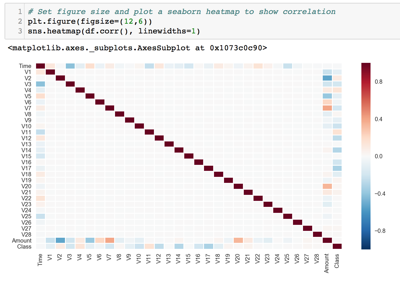
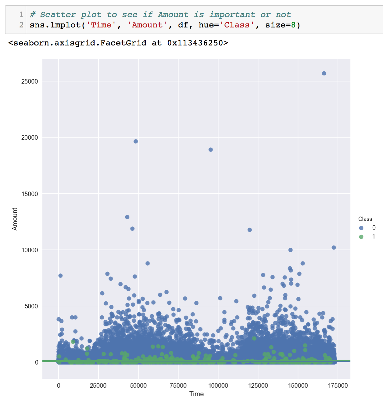
As we expected, there were no correlation between any of the V features, which is great. Here, we can also get an intuition which V feature correlates with the Class column. We might make use of this information for feature selection/engineering later.
The Time VS Amount plot revealed that Amount might not be a strong indicator of fradulent transactions. As we can see, most of the green dots (fraud) fall below ~2500. Much of the non-fraud cases are also below that amount.
Let’s take a closer look at each of our features now. I ran a loop to make distribution plots for every V feature. There are a total of 28 plots, so I shall not clutter this page with them (click here) to view the Jupyter Notebook).
Finally, we get to our Class labels. A simple bar plot was created, and the percentage fraud was calculated.
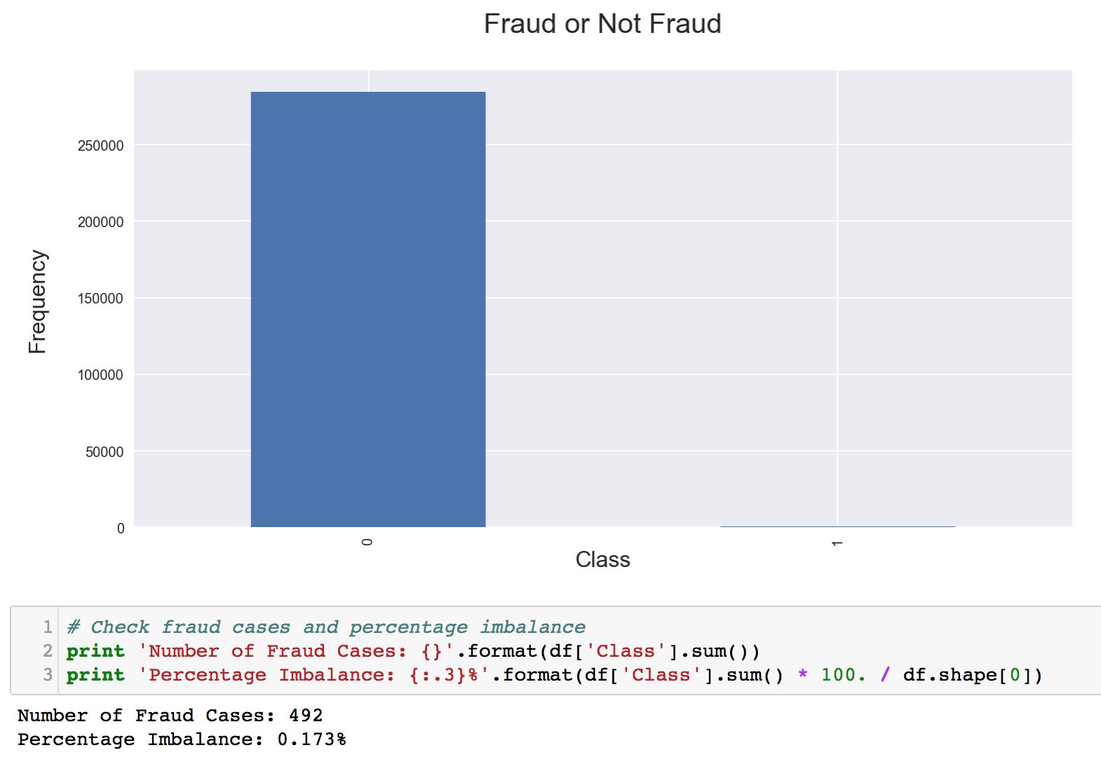
What an imbalanced dataset! Out of over 280,000 rows, only 492 are fraudulent transactions. That equates to about 0.173%. Isn’t that akin to finding a needle in a haystack?
What does this mean? Having a ratio like this, we must know that we cannot make use of conventional/traditional accuracy measures as our performance metric. In fact, even our approach to sampling and modelling will be very different.
Simple accuracy scores are not feasible because even a dumb machine, which predicts non-fraud all the time, will get our baseline accuracy score of 100.0 - 0.173 = 99.827%! This might appear awesome as an article headline (thus, please remember to always be critical when reading/evaluating articles), but it is far from the truth. It does not help at all in understanding how our model performs in detecting fraud cases.
What do we do then? We make use of precision and recall scores to help us evaluate our models. Recall (rate of False Negative) refers to how many actual frauds we are able to detect. Whereas, Precision (False Positive) refers to how many of our machine’s predicted fraud cases are real, actual frauds. Ideally, we want to get high scores for both of them. However, reality is hardly kind. In this case of Credit Card Fraud, recall scores are more crucial. If a transaction is fraudulent and we predict it as normal, the consequence is much greater than if we predict a normal case as fraud. Therefore, our main focus will be on recall scores, but of course, we will also optimize the precision score, and allow our models to ‘tune’ between placing emphasis on either. Flexibility!
Manual Undersampling
We'll try a simple manual undersampling of the over-represented class first, by randomly selecting 492 rows out. We would now have 492 fraud and 492 normal transactions. We then prepare both of our datasets (whole data and undersampled data) by splitting them into train and test sets for further usage. A basic Logistic Regression is used to model on the undersampled data.


Logistic Regression on Under-Sampled Data
A gridsearch was performed to obtain the best hyperparameters for the model. We will be predicting on 3 sets of data.
- Undersampled Test Set
- Whole Data Test Set
- Lastly, we try to train on the whole data, and predict to see how it goes!
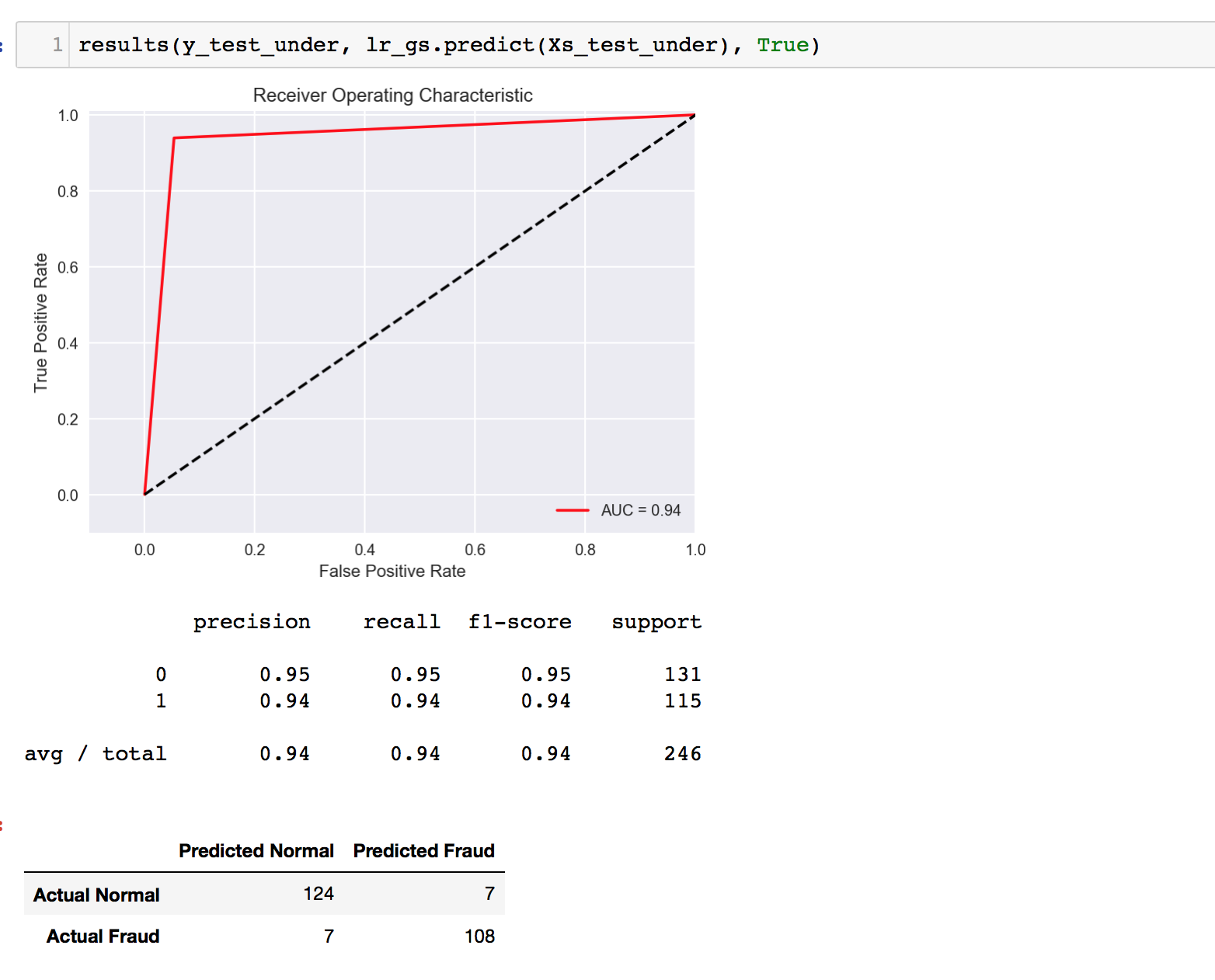
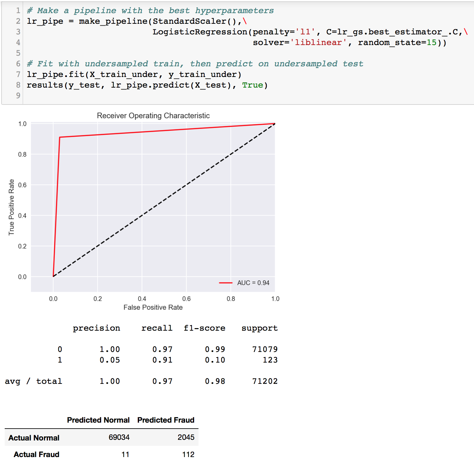
It comes without surprise that the model performs well on its own undersampled test set. However, it feels quite impressive that it managed to achieve a pretty high recall score of 0.91 on the whole dataset! Granted, the precision score leaves quite a lot to be desired, but, we must remember that this is merely a Logistic Regression model on 984 data points (undersampled). I’d say it did really well for its simplicity. Of course, we would not be stopping here. Regardless, this result is aligned with the direction we’re headed; a heavier focus on recall.
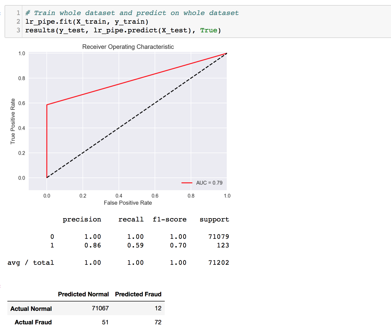
For the last model, we trained the entire data set and predicted. As expected, the scores are not good, as the training set is in itself imbalanced at 0.173%. We are missing out at least 40% of all fraudulent transactions here. That’s a significant impact in the real world. This model was done just for constrastive purposes to illustrate the importance of sampling techniques on imbalanced datasets. Even a simple small scale undersampling gave us a much higher recall score.
More Modelling with IMBLearn Sampling Techniques
IMBLearn (short for imbalanced-learn) is a python package offering a number of re-sampling techniques commonly used in datasets showing strong between-class imbalance. It is compatible with scikit-learn and is part of scikit-learn-contrib projects. For more information, please visit the documentation.
The first technique we will try is the popular SMOTE, which means Synthetic Minority Over Sampling Technique. SMOTE has proven effectiveness over lots of applications, and several papers/articles have had success with it. What SMOTE does is that it constructs synthetic samples from the under-represented class by making use of nearest neighbours. It is sort of a bootstrapping method. Therefore, in our case, the train set has about 213,000 rows. SMOTE will use the 492 fraud data points as reference to create synthetic samples up to the number of rows of the over-represented class, which is ~213,000 (to get 50/50 ratio).

After SMOTE’ing, we perform the usual gridsearch to find hyperparameters for the subsequent Logistic Regression model. We always start modelling with Logistic Regression because it is the simplest model and can serve as a baseline for us to understand how the dataset fares. In addition, if Logistic Regression happens to be sufficient in giving us good scores, we could just stick with it! Simplicity is beauty.
This time, due to having much more rows (over 400,000), the gridsearch process had to take about 30 minutes to complete. The results were ‘underwhelming’ though. It seemed like the value of C does not really change the score, which hangs around 0.94 all the time. We must be reminded though, that the score reflected through gridsearch is not precision or recall but a simple accuracy measure. Thus, it may not be reliable after all in our case. In fact, I had to manually run an empirical analysis to determine a decent C value, which was also ‘underwhelming’ because they do not have significant differences. As a result, I decided on a smaller C value for computation speed.
Hereon, we will make use of pipelines for cleaner code and ease of operations as we would be running many models. It is important to note that IMBLearn’s pipeline is different from that of sklearn’s. The latter is unable to accept the former’s sampling technique as part of its pipeline. Thus, please make sure you are importing and using IMBLearn’s pipeline.
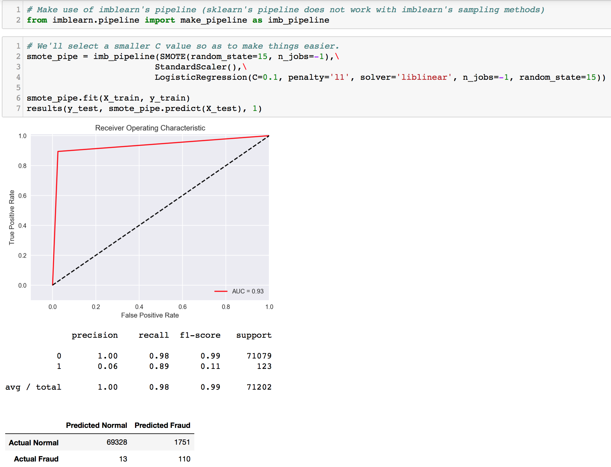
Recall score seemed to maintain (in comparison to our ‘benchmark’ undersampling LR earlier), but a slight improvement was observed in precision. Unfortunately, that is not our main goal at this point. Let’s move on to try other sampling techniques. The next will be Edited Nearest Neighbours (ENN undersampling).
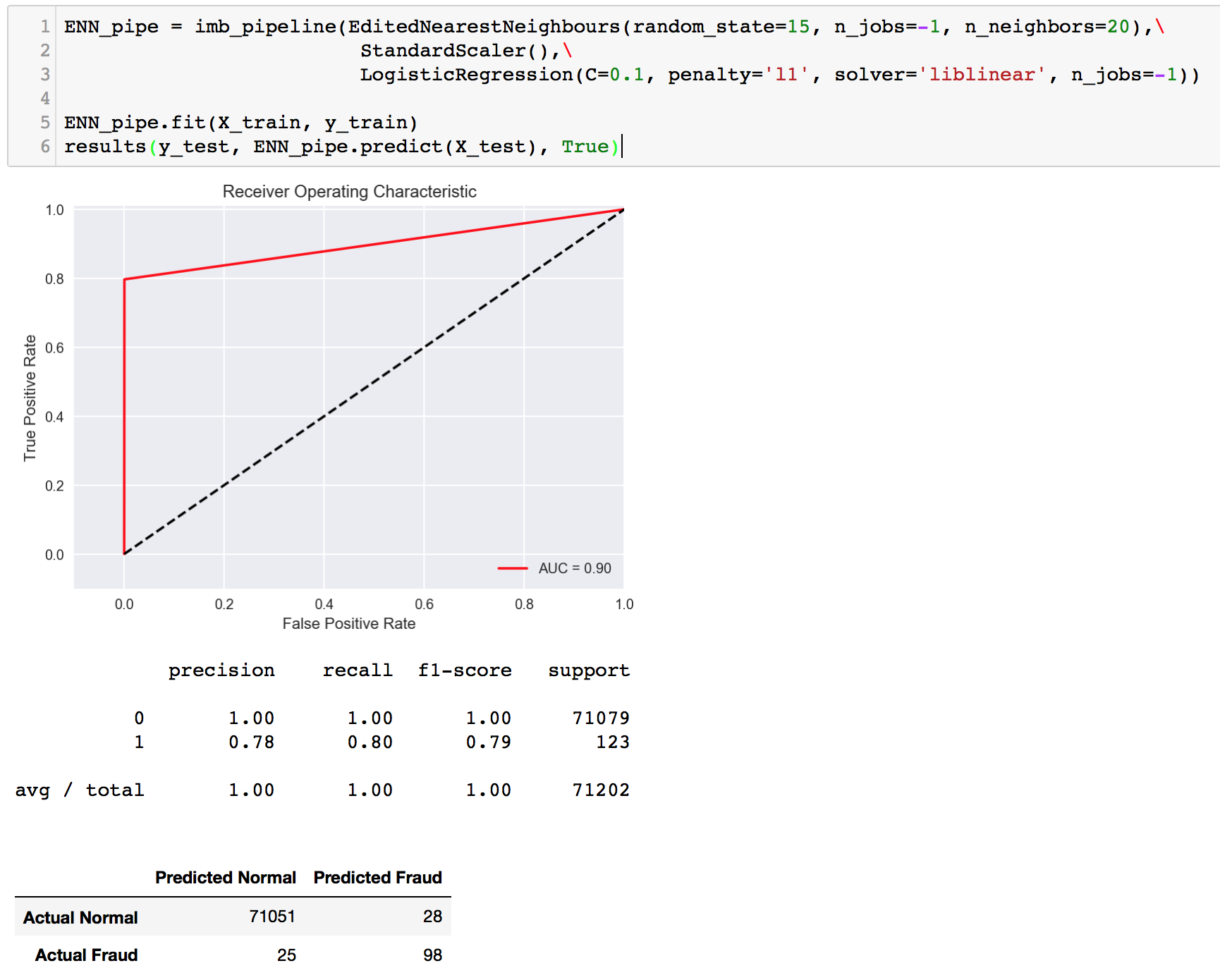
Wow! This is the first time we’re seeing double digits for both our FP and FN. The recall score is not as high as before, but the precision score flew up to about 80%; very close to our recall. While these scores might seem very balanced and fairly high, we should not be satisfied because our goal is to maximize recall. Here, we are still missing out on ~20% of frauds. Now, how about we combine SMOTE and ENN? It’s SMOTEENN time.
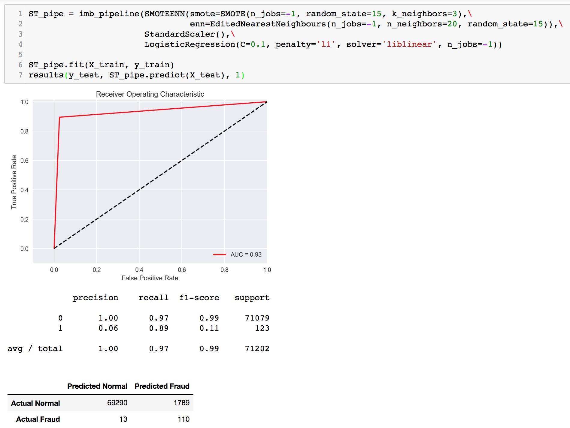
Well, a combination of both did not give us much difference in results. Let’s a take a step further and adjust the probability thresholds to see if it is possible to balance FP and FN. By using .predict_proba(), the probability values for a data point to be Class 0 or 1 are provided. We can turn it into a dataframe, and add a new column for our manual prediction that is based on adjusting the threshold. For example, if data point 100 has a probability of 0.65 to be Class 1, the default threshold of 0.5 will classify this point as 1. If we adjust the threshold to be 0.7 (which is higher than the probability value), the data point will be classified as 0 since it is below 0.7.
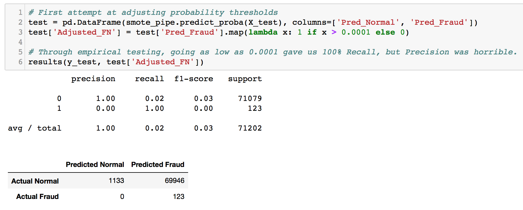
Through empirical testing, we found that the threshold (for our SMOTE model) had to be 0.0001 in order to achieve 100% recall. However, it came at a severe cost on precision. Given these values, the machine might as well predict every point as fraud! Moving on, we will be adjusting thresholds often, so, we built a function for it.
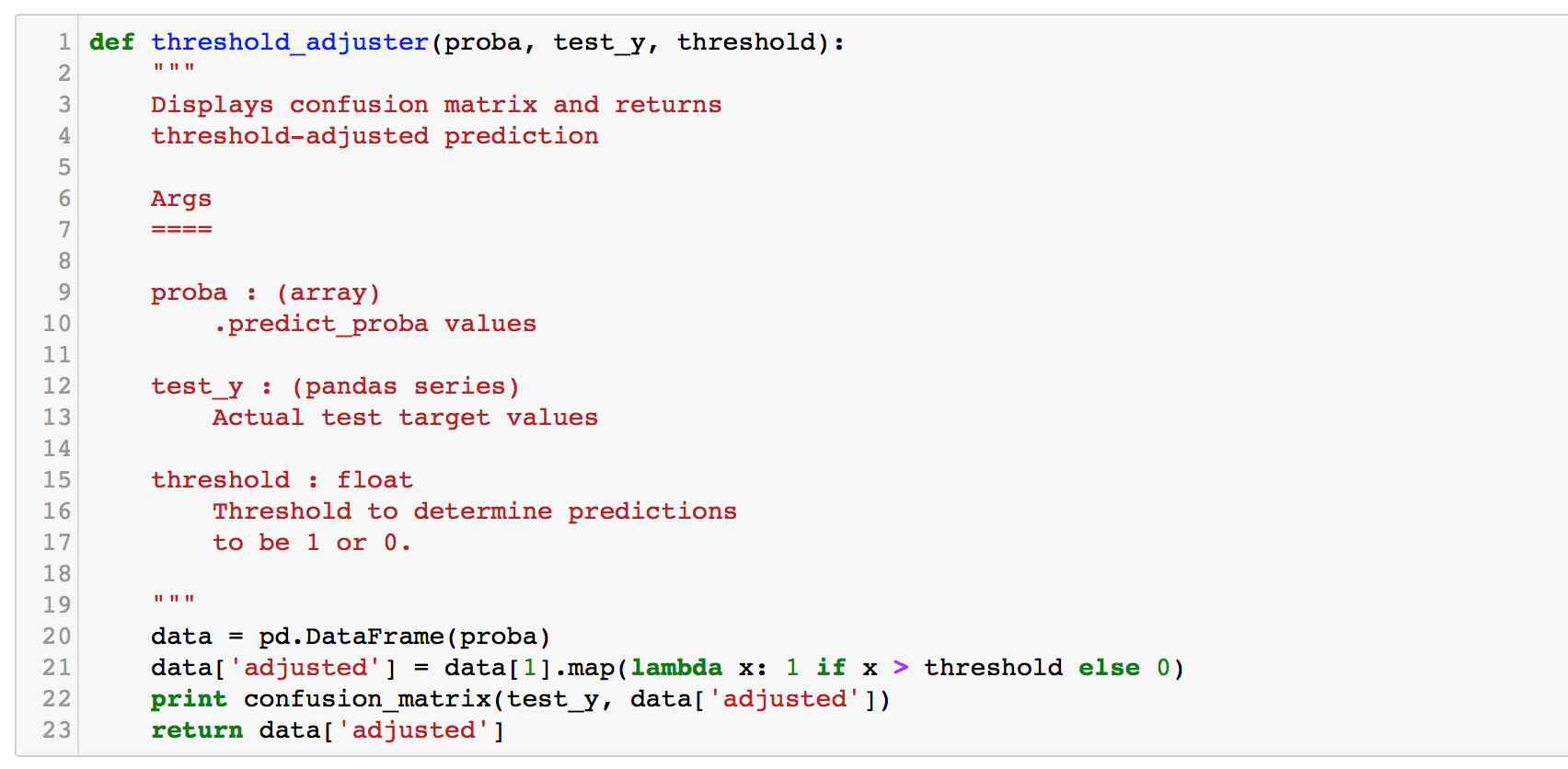
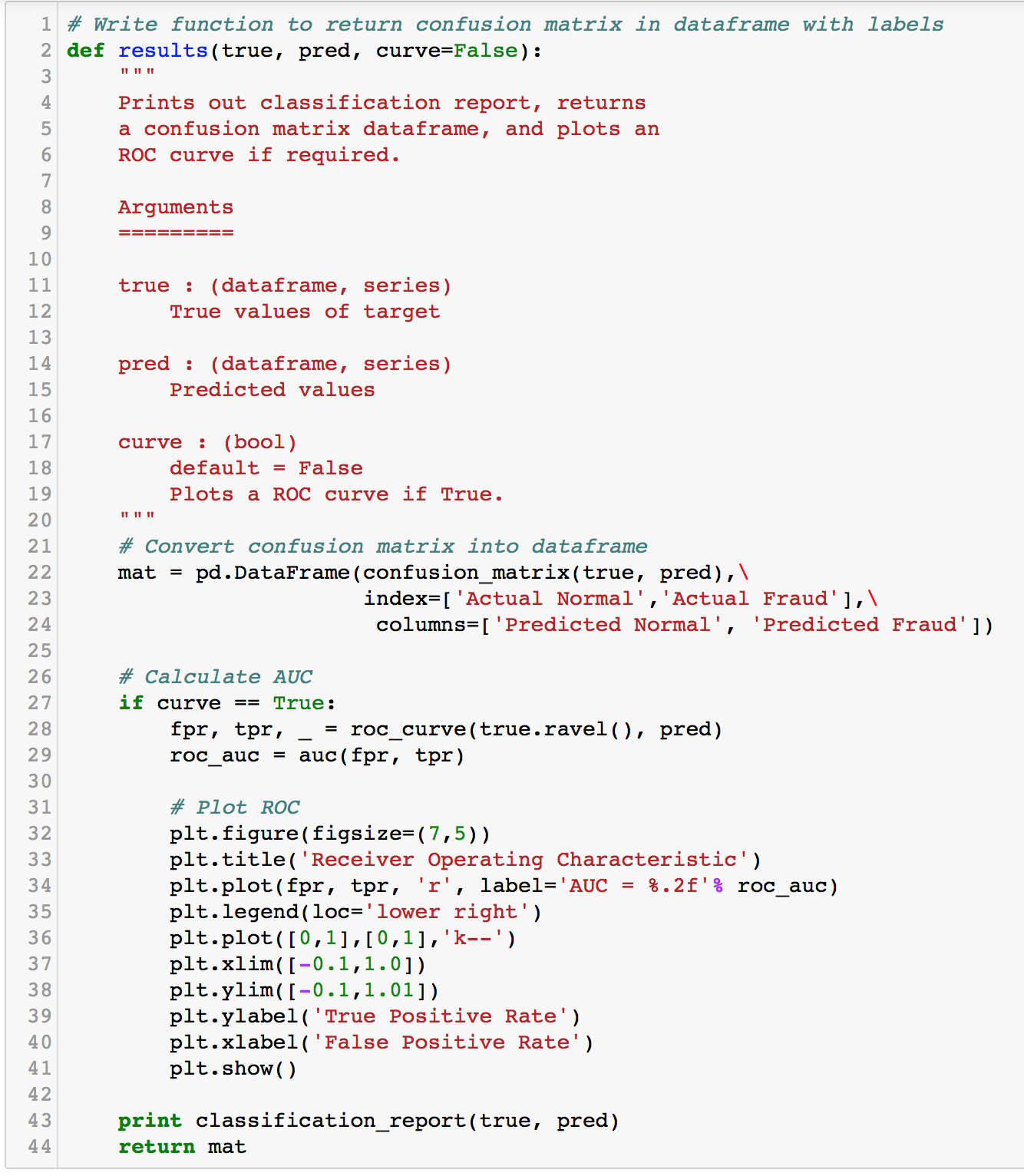
The function takes in the .predict_proba() values, the true y values, and a user-specified threshold value. It prints out the confusion matrix and returns the adjusted prediction values of 0 and 1.
Random Forests
I tried to run a gridsearch which took hours overnight and crashed the kernel. Thereafter, I manually tested several parameters and found these to produce better results.
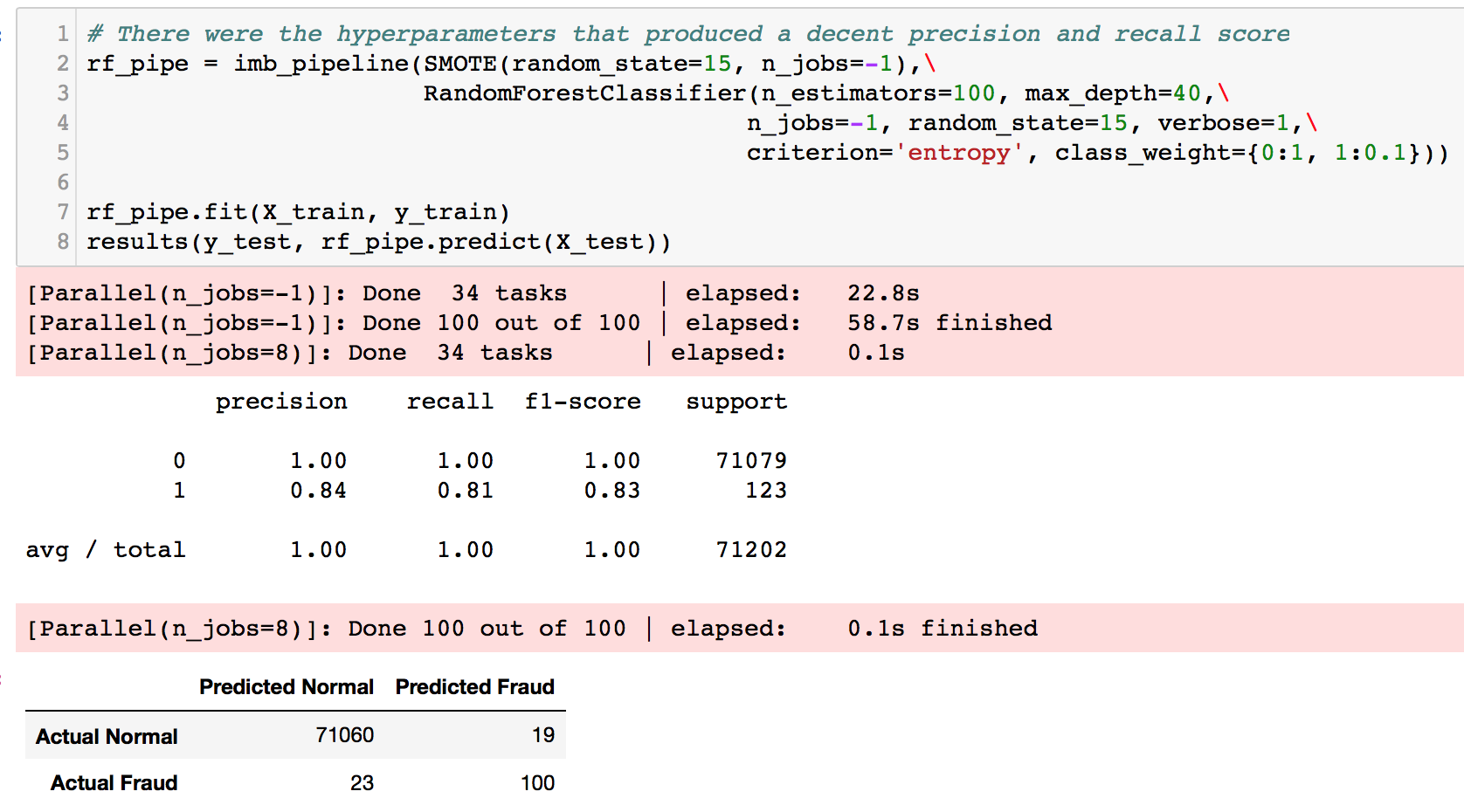
We get slightly better recall and precision scores at least ~0.80 each. However, the same problem remains. The results do not match our goal in minimizing recall scores and False Negatives. Next, we try to train a RF on our manually undersampled data.

Let's see if we can get a better score by merging these two models together; ensembling. Both model's predicted probabilities are added together and averaged. Then, the threshold is adjusted to see how the model does in terms of precision vs recall.
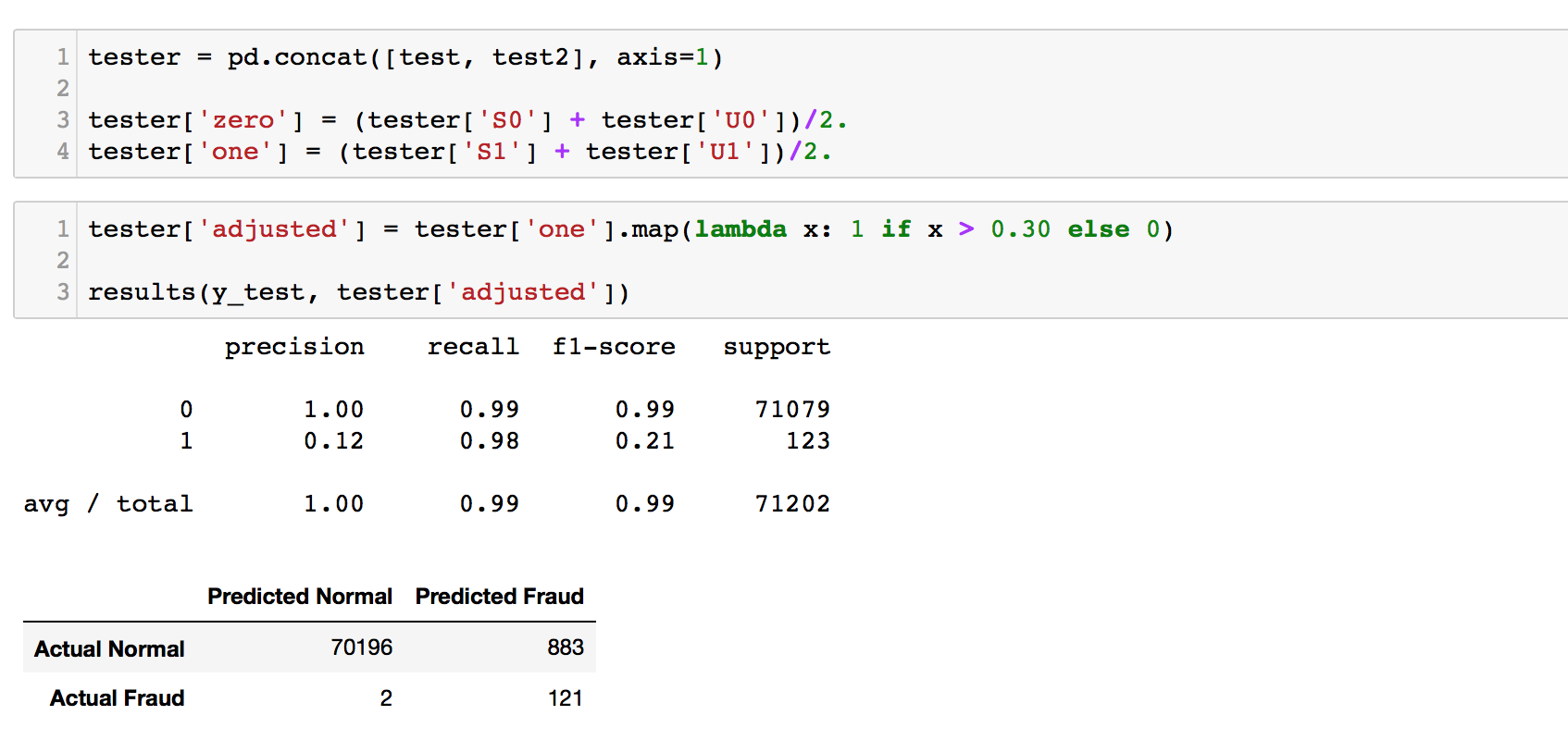
An ensemble of both models did give us an improvement! The recall score remained from the undersampled model (2 FN), and the precision was improved quite significantly to 0.12, at 883 False Positives. This looks promising. We will attempt even more ensembling later to boost our scores.
eXtreme Gradient Boosting XGBoost
We have come to the powerhouse. Please visit XGBoost documentation for more information! As before, we will be sampling with imblearn.
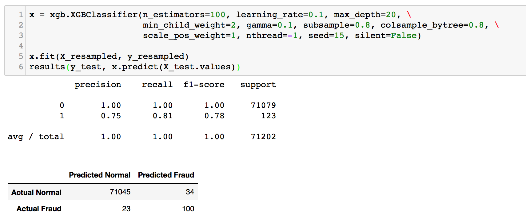
Still, there does not seem to be a significant improvement in the scores. Note that we have not performed extensive parameter tuning yet.
So far, we have tried Logistic Regression, Random Forest, and XGBoost together with a handful of sampling techniques. Our best score was 98% recall and 12% precision which was achieved through a two-model ensemble of Random Forest (trained on whole data and undersampled data). It's time to reach deeper into ensembling.
Ensembling Sampling
Essentially, this is just re-sampling of the undersampled dataset. Our first sampling technique above was a manual under-sampling of 492 data points from the over-represented class. This gave us a dataset of 984 points, with a 50/50 ratio of fraud/normal, where all the fraud data points are included.
Now, we want to train more models in order to ensemble them, which is, to merge their results and get a 'majority vote'. It is like listening to several experts and aggregating their wisdom. With this kind of 'community voting', we hope something better will emerge.
How does this happen? Similar to before, we randomly select 492 rows from the over-represented class, join it with our 492 fraud cases, and here we have one dataset for training. We repeat this process for k number of times. Each time, we will be getting different sets of 492 normal transactions. Therefore, we will have k number of datasets and each of them will be modelled separately. We then take each individual model's prediction, ensemble them, and acquire new predictions! For example, we can do this 10 times for Logistic Regression, 10 times for Random Forests, and 10 times for XGBoost, then ensemble them. The possibilities are endless.
How can we build on that? We can even refine this further by altering the class ratio within each dataset. Currently, all k of our datasets have a 50/50 class ratio. We can tune that by having some datasets contain class ratio of 25/75, 40/60 etc. This way, the weights for each class will vary in different trained models, and perhaps giving us a more balanced outcome when testing.
We will be running an ensemble model plus an ensemble model with ratio adjustment on all methods we have tried above; Logisitic Regression, Random Forest, and XGBoost.
Logistic Regression Ensemble Sampling
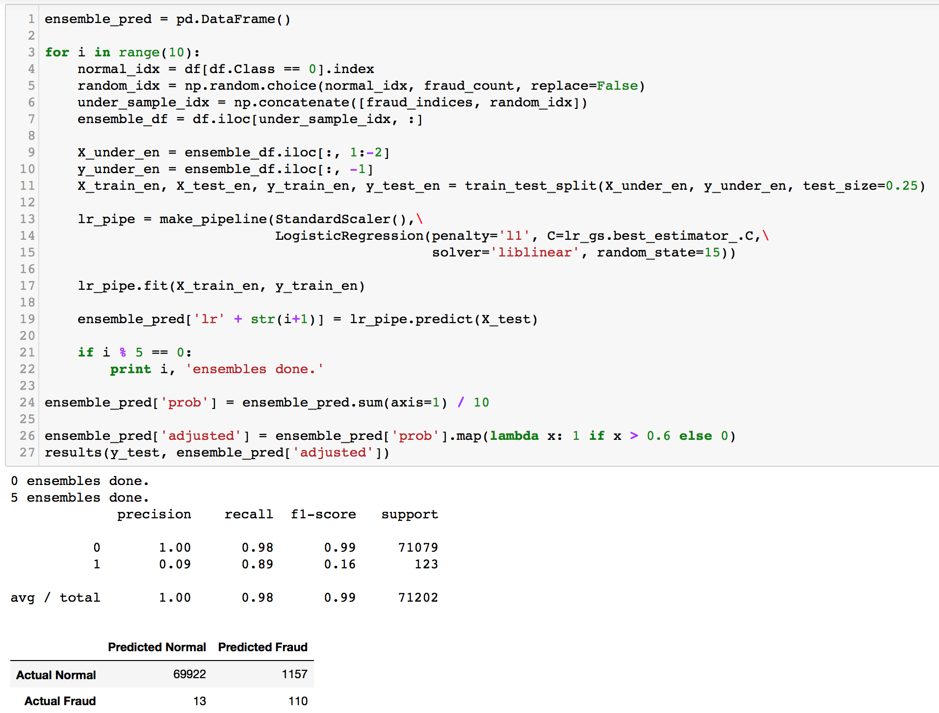
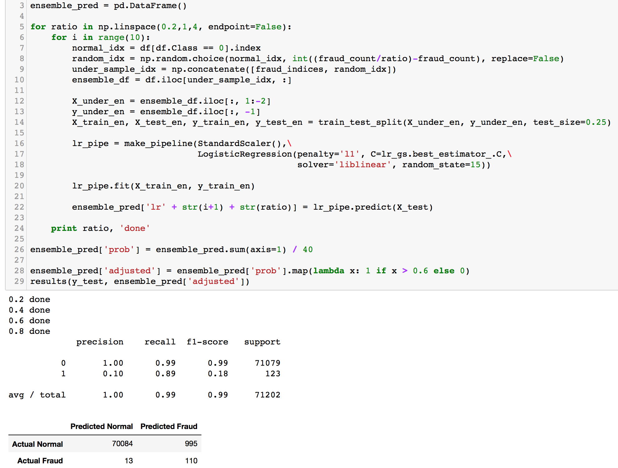
Gradual improvement! Our first ensemble model did better than its single counterpart by a reduction of about 900 False Positives and gave a precision score of about 0.09. Recall score did not change though. After ensembling, the precision score increased slightly. Things are looking good. Random Forest and XGBoost should perform much better than this.
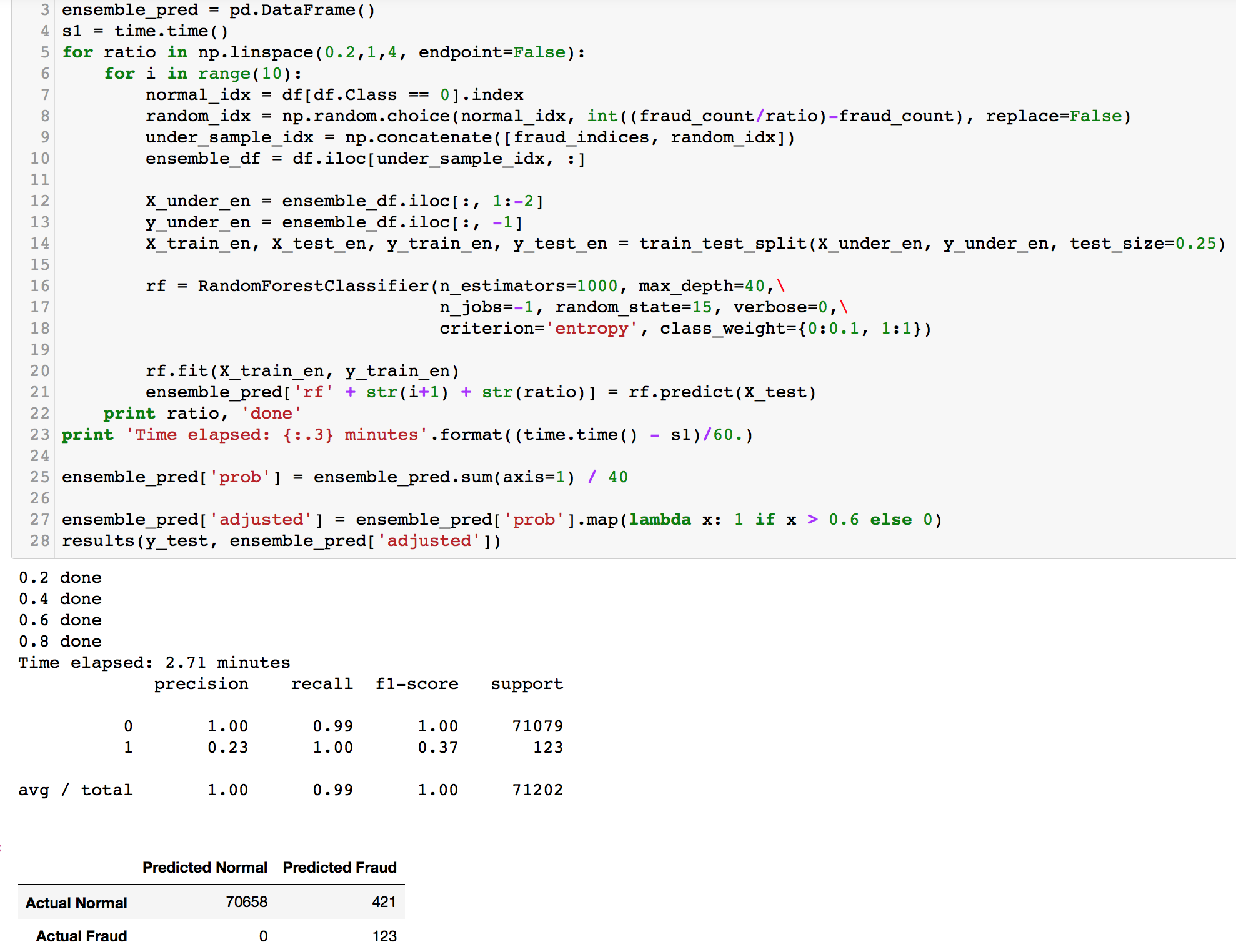
Random Forest Ensemble Sampling Our Forest hyperparameters were obtained through empirical testing and gridsearch. The class weight was set to 0.1 for the normal class (0) as we want the model to place more weights on our fraud cases (1). We don't want to miss out any fraud cases.
XGBoost Ensemble Sampling
Auto-Encoder Neural Network
