Recommender System

November 17, 2017

For details and code, please visit my Jupyter Notebook.

This is my capstone project for the Data Science Immersive program at GA. The program is a 12-week full-time course with five projects in total. It covers a very wide range of Data Science topics, but unfortunately for me, Recommender Systems were only covered for about half a day, in week 11! Therefore, the entire project was pretty much a self-learning journey, from scratch.

Objective

The aim of this project is to dive into the world of Recommender Systems, and explore various methods for Collaborative Filtering. The focus will be on understanding the math and algorithm behind them, then applying them to generate recommendations. Although I chose book reviews, it does not actually matter what the rated item is. Collaborative Filtering is based on seeking similar reviews amongst users/items, and predicting ratings from the existing ratings themselves. Therefore, it is considered item-agnostic.

Data

Data: Amazon's Product Review and Data, 1996 - 2014
File: gzip file containing json within

The dataset consists of over 142 million reviews, of which 22 million are book reviews.
However, I will only be using about 100 thousand book reviews due to time/memory constraints,
by setting a minimum of 40 reviews for each book (item) and each user.

Reference (source of data):
R. He, J. McAuley. Modeling the visual evolution of fashion trends with one-class collaborative filtering. WWW, 2016

Clean and Prepare Data

The gzip data is loaded with the following functions. It takes a while to process, so, it is recommended to pickle the dataframes after loading.

	def parse(path):
   		g = gzip.open(path, 'rb')
    	for l in g:
        	yield eval(l)

	def getDF(path):
    	i = 0
    	df = {}
    	for d in parse(path):
        	df[i] = d
        	i += 1
    	return pd.DataFrame.from_dict(df, orient='index')
	

	def downsize(df, u_col, i_col, min_r_count):
    	"""
    	Takes in a dataframe that includes columns "user", "item", "ratings"
    	and returns a new dataframe where users and items each have a
    	minimum amount of ratings as specified.

    	Arguments
    	=========
    
    	df : (dataframe)
        	Dataframe that has columns User, Item, and Ratings
        
    	u_col: (string)
        	Name of User Column
        
    	i_col: (string)
        	Name of Item Column

    	min_r_count: (int)
        	Mininum number of ratings for each user and item
        
    	"""
    	size = df.shape[0]
    	while True:
        	user5 = df.groupby(u_col).size().reset_index(name='count')
        	user5 = user5[user5['count'] < min_r_count]
        	df = df[~df[u_col].isin(user5[u_col])]

        	item5 = df.groupby(i_col).size().reset_index(name='count')
        	item5 = item5[item5['count'] < min_r_count]
        	df = df[~df[i_col].isin(item5[i_col])]
        	print df.shape
       		if df.shape[0] == size:
            	break
        	else:
            	size = df.shape[0]
    	print df[u_col].nunique(), 'users'
    	print df[i_col].nunique(), 'items'
    	return df
	

Train-Test Split

In most traditional Machine Learning applications, train-test splits can be performed by simply separating a random selection of rows in the data. However, in Collaborative Filtering, that would not work because we will need all users to be in both train and test sets. If we randomly take rows out, we will lose a batch of users.

Therefore, what we need to do is to mask/remove some ratings for every user on the train set. There are a few ways to do this. In this case, we will split a user's ratings into two. This means, if a user has rated 40 items, the train set would have 25, and the test, 15. The ratings do not overlap, and both train and test sets are disjoint.

def train_test_split(ratings, size):
    test = np.zeros(ratings.shape)
    train = ratings.copy()
    for user in xrange(ratings.shape[0]):
        test_ratings = np.random.choice(ratings[user, :].nonzero()[0], 
                                        	size=size, replace=False)
        train[user, test_ratings] = 0.
        test[user, test_ratings] = ratings[user, test_ratings]
        
    # Test and train are truly disjoint
    assert(np.all((train * test) == 0)) 
    return train, test

Matrix Factorization using ALS and SGD

For matrix factorization, we have two sets of latent vectors to solve, the user and the item. In Alternating Least Squares, we hold one set of latent vectors constant and we solve for the other non-constant vector. Now this is the alternating part. Once we have this solved vector, we now hold this newly solved vector constant, and then solve again for the new non-constant vector (which was the previous constant). This is done repeatedly until convergence.

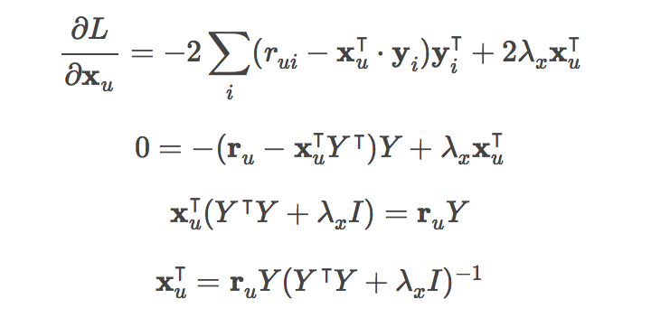
That was ALS. Now, let's move on with Stochastic Gradient Descent (SGD). In SGD, we also take the derivative of the loss function, but now it is with respect to each variable in the model. The derivative is taken and feature weights are updated one individual sample at a time.
In our SGD model, we will also include biases for each user and item, and a global bias. For example, some users might have a high average rating, or that certain items might have an average rating that is less than the global average. We would want to attempt to address this by adding biases.

Now that we have our equations, let's proceed to the computation.

class MatFac():
    def __init__(self, 
                 ratings,
                 n_factors=40,
                 optimize='sgd',
                 item_fact_reg=0.0, 
                 user_fact_reg=0.0,
                 item_bias_reg=0.0,
                 user_bias_reg=0.0,
                 verbose=False):
        """
        Matrix factorization model to predict empty entries in a matrix. 
        Ratings matrix should be in the format: User x Item.
        
        Arguments
        =========
        ratings : (ndarray)
            User x Item matrix with ratings
        
        n_factors : (int)
            Number of latent factors to use in the model
            
        optimize : (str)
            Method of optimization. Options include 
            'sgd' or 'als'.
        
        item_fact_reg : (float)
            Regularization term for item latent factors
        
        user_fact_reg : (float)
            Regularization term for user latent factors
            
        item_bias_reg : (float)
            Regularization term for item biases
        
        user_bias_reg : (float)
            Regularization term for user biases
        
        verbose : (bool)
            Whether or not to print out training progress
        """
        
        self.ratings = ratings
        self.n_users, self.n_items = ratings.shape
        self.n_factors = n_factors
        self.item_fact_reg = item_fact_reg
        self.user_fact_reg = user_fact_reg
        self.item_bias_reg = item_bias_reg
        self.user_bias_reg = user_bias_reg
        self.optimize = optimize
        if self.optimize == 'sgd':
            self.sample_row, self.sample_col = self.ratings.nonzero()
            self.n_samples = len(self.sample_row)
        self._v = verbose

    def als_step(self,
                 latent_vectors,
                 fixed_vecs,
                 ratings,
                 _lambda,
                 type='user'):
        """
        One of the two ALS steps. Solve for the latent vectors
        specified by type.
        """
        if type == 'user':
            YTY = fixed_vecs.T.dot(fixed_vecs)
            lambdaI = np.eye(YTY.shape[0]) * _lambda

            for u in xrange(latent_vectors.shape[0]):
                latent_vectors[u, :] = solve((YTY + lambdaI), 
                                             ratings[u, :].dot(fixed_vecs))
        elif type == 'item':
            XTX = fixed_vecs.T.dot(fixed_vecs)
            lambdaI = np.eye(XTX.shape[0]) * _lambda
            
            for i in xrange(latent_vectors.shape[0]):
                latent_vectors[i, :] = solve((XTX + lambdaI), 
                                             ratings[:, i].T.dot(fixed_vecs))
        return latent_vectors

    def train(self, n_iter=10, learning_rate=0.1):
        """ Train model for n_iter iterations from scratch."""
        # initialize latent vectors        
        self.user_vecs = np.random.normal(scale=1./self.n_factors,\
                                          size=(self.n_users, self.n_factors))
        self.item_vecs = np.random.normal(scale=1./self.n_factors,
                                          size=(self.n_items, self.n_factors))
        
        if self.optimize == 'als':
            self.mini_train(n_iter)
        elif self.optimize == 'sgd':
            self.learning_rate = learning_rate
            self.user_bias = np.zeros(self.n_users)
            self.item_bias = np.zeros(self.n_items)
            self.global_bias = np.mean(self.ratings[np.where(self.ratings != 0)])
            self.mini_train(n_iter)
    
    
    def mini_train(self, n_iter):
        """ 
        Train model for n_iter iterations. Can be 
        called multiple times for further training.
        """
        ctr = 1
        while ctr <= n_iter:
            if ctr % 10 == 0 and self._v:
                print '\tcurrent iteration: {}'.format(ctr)
            if self.optimize == 'als':
                self.user_vecs = self.als_step(self.user_vecs, 
                                               self.item_vecs, 
                                               self.ratings, 
                                               self.user_fact_reg, 
                                               type='user')
                self.item_vecs = self.als_step(self.item_vecs, 
                                               self.user_vecs, 
                                               self.ratings, 
                                               self.item_fact_reg, 
                                               type='item')
            elif self.optimize == 'sgd':
                self.training_indices = np.arange(self.n_samples)
                np.random.shuffle(self.training_indices)
                self.sgd()
            ctr += 1

    def sgd(self):
        for idx in self.training_indices:
            u = self.sample_row[idx]
            i = self.sample_col[idx]
            prediction = self.predict(u, i)
            e = (self.ratings[u,i] - prediction) # error
            
            # Update biases
            self.user_bias[u] += self.learning_rate * \
                                (e - self.user_bias_reg * self.user_bias[u])
            self.item_bias[i] += self.learning_rate * \
                                (e - self.item_bias_reg * self.item_bias[i])
            
            # Update latent factors
            self.user_vecs[u, :] += self.learning_rate * \
                                    (e * self.item_vecs[i, :] - \
                                     self.user_fact_reg * self.user_vecs[u,:])
            self.item_vecs[i, :] += self.learning_rate * \
                                    (e * self.user_vecs[u, :] - \
                                     self.item_fact_reg * self.item_vecs[i,:])
    def predict(self, u, i):
        """ Predict rating for single user and item."""
        if self.optimize == 'als':
            return self.user_vecs[u, :].dot(self.item_vecs[i, :].T)
        elif self.optimize == 'sgd':
            prediction = self.global_bias + self.user_bias[u] + self.item_bias[i]
            prediction += self.user_vecs[u, :].dot(self.item_vecs[i, :].T)
            return prediction
    
    def predict_all(self):
        """ Predict ratings for all user and item."""
        predictions = np.zeros((self.user_vecs.shape[0], 
                                self.item_vecs.shape[0]))
        for u in xrange(self.user_vecs.shape[0]):
            for i in xrange(self.item_vecs.shape[0]):
                predictions[u, i] = self.predict(u, i)
                
        return predictions
    
    def calculate_learning_curve(self, iter_array, test, learning_rate=0.1):
        """
        Keep track of RMSE as a function of training iterations.
        
        Params
        ======
        iter_array : (list)
            List of numbers of iterations to train for each step of 
            the curve. e.g. [1, 5, 10, 20]
        test : (2D ndarray)
            Test dataset (user x item).
        
        The function creates two new class attributes:
        
        train_rmse : (list)
            Training data RMSE values for each value of iter_array
        test_rmse : (list)
            Test data RMSE values for each value of iter_array
        """
        iter_array.sort()
        self.train_rmse =[]
        self.test_rmse = []
        iter_diff = 0
        for (i, n_iter) in enumerate(iter_array):
            if self._v:
                print 'Iteration: {}'.format(n_iter)
            if i == 0:
                self.train(n_iter - iter_diff, learning_rate)
            else:
                self.mini_train(n_iter - iter_diff)

            predictions = self.predict_all()

            self.train_rmse += [get_rmse(predictions, self.ratings)]
            self.test_rmse += [get_rmse(predictions, test)]
            if self._v:
                print 'Train RMSE: ' + str(self.train_rmse[-1])
                print 'Test RMSE: ' + str(self.test_rmse[-1])
            iter_diff = n_iter

We'll run this by choosing 50 latent vectors, learning rate 0.001, and without regularization. Let's see how this performs from the plot below.

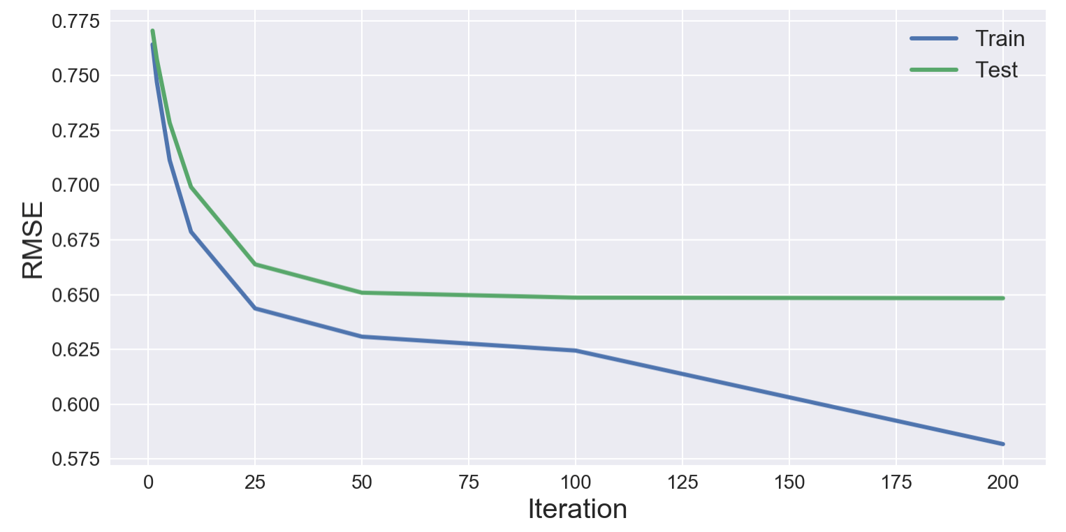
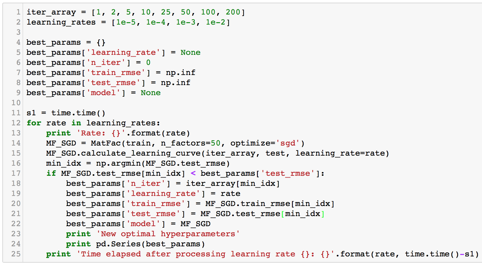
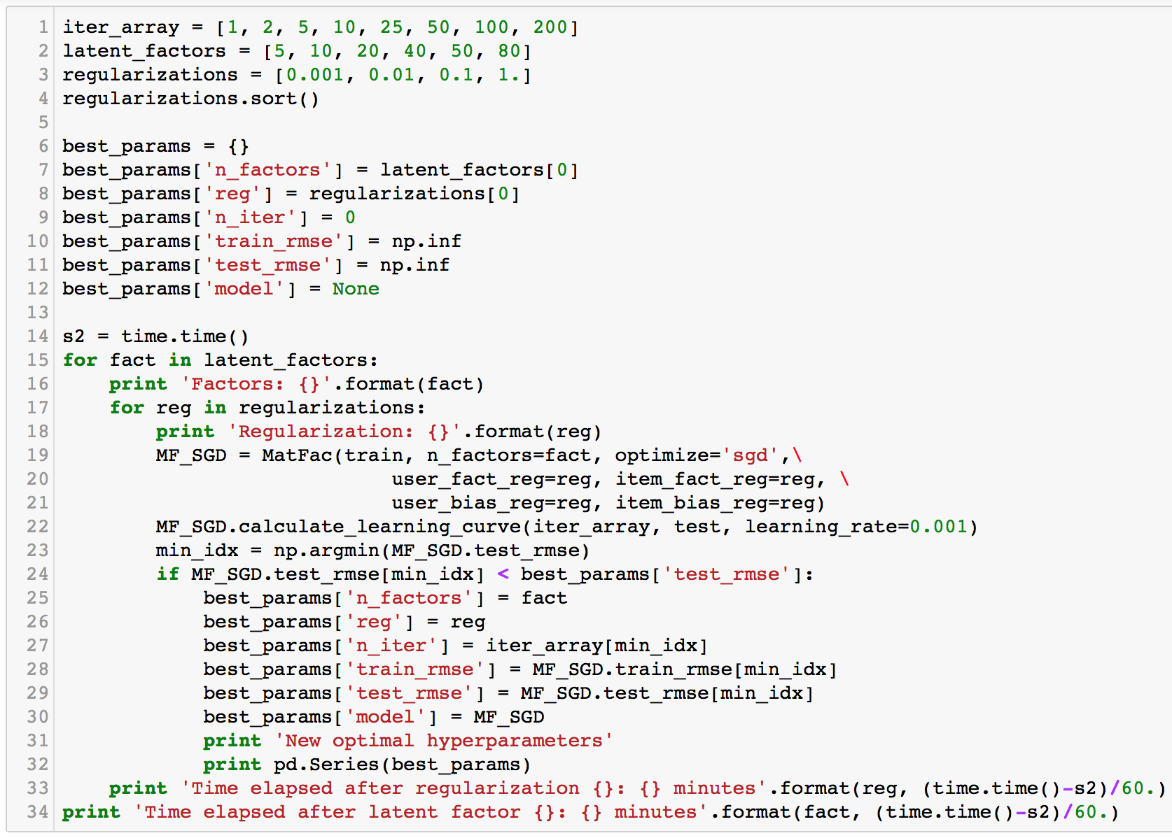
Now that the model is working well, let's try to take it a little further by finding the best hyperparameters. It's like a manual gridsearch in our case.

• learning rate
• latent factors
• regularization (keeping it same for user and item)

Best hyperparameters:

• learning rate: 0.001
• latent factors: 50
• regularization: 0.001
• iterations: 200

It’s time to run our model to generate predictions, and recommendations.
The first impression I had when I ran it was that I knew nothing about the recommended books. I had no intuition at all, and had to look them up. Interestingly, they do belong to a similar category. Most of them were Literature/Fiction, and Romance. Let’s look at the recommendations for two users; user1 has the most ratings, and user2, the least.

User1

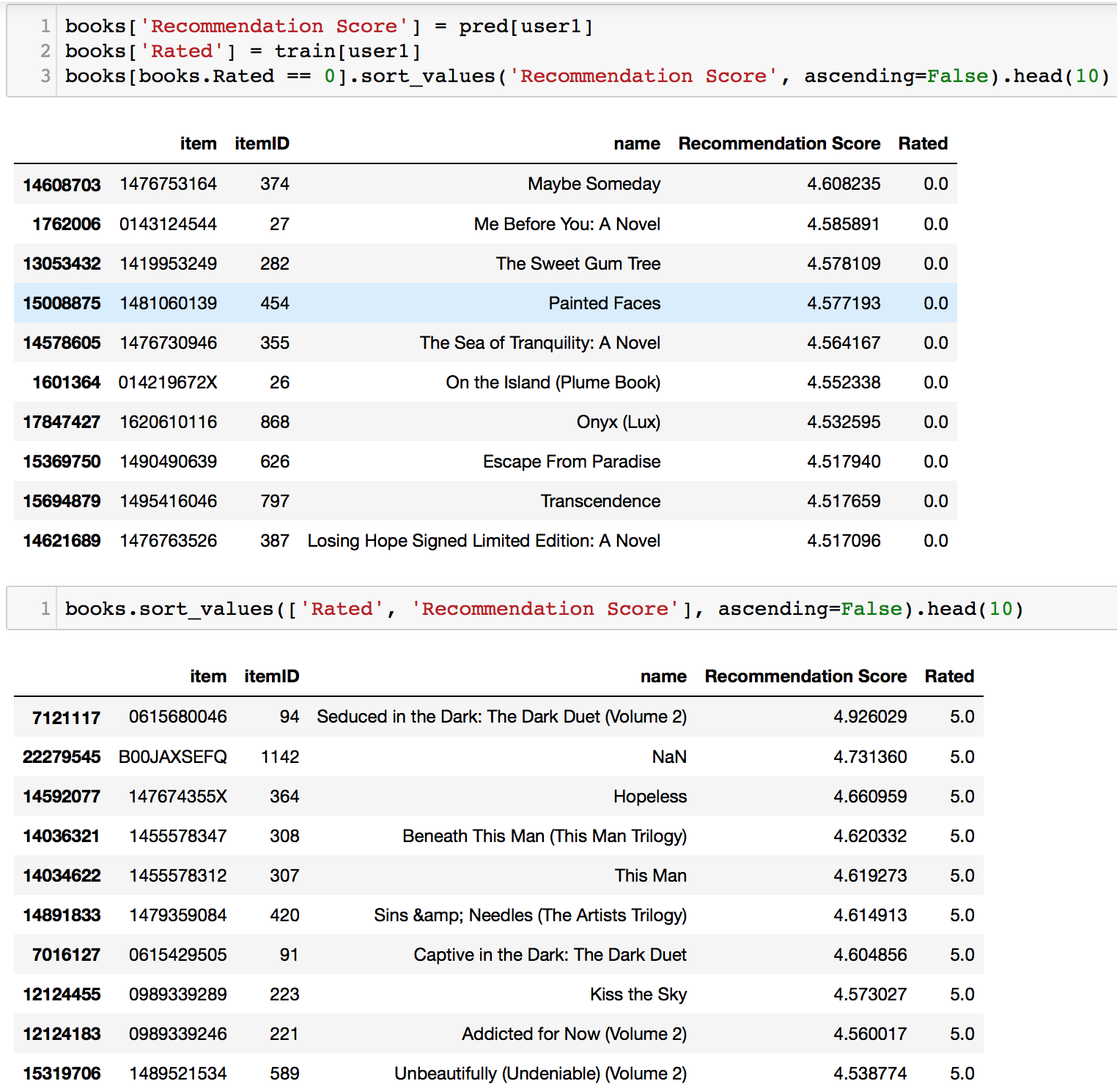
The books here shown for User1 mostly fall under Romance/Women’s books. We can also compare our model’s predicted score to the user’s actual ratings in the second table as well.

User2

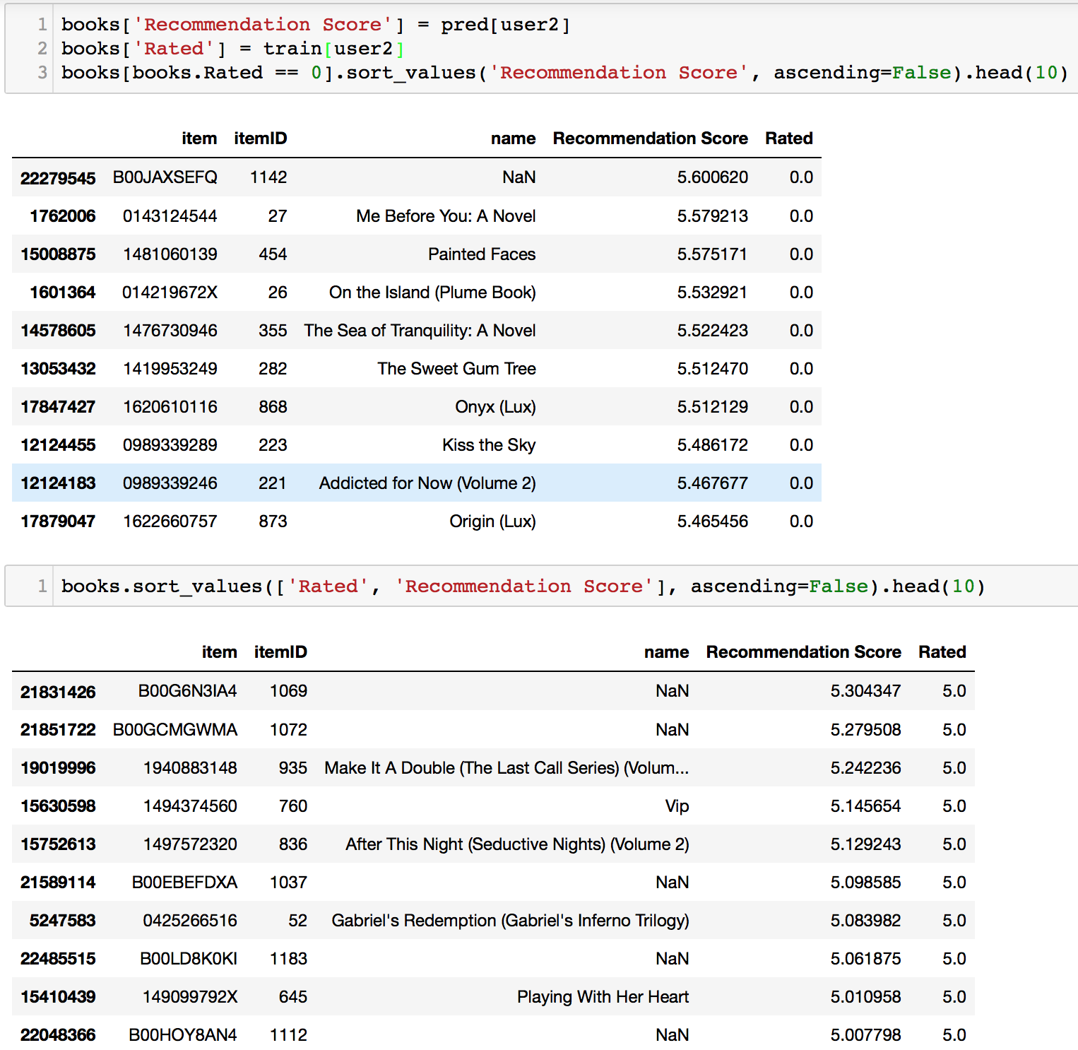
Coincidentally, the books that user2 has rated belong to Romance as well. Our model’s recommendations did well here too, having mostly books in the Romance category.

Conclusion
I performed Matrix Factorization by optimizing through Alternating Least Squares (ALS) and (SGD). The RMSE results were great. At 0.648, this means that all of our predictions are only 0.648 away from the actual ratings, on average. The model's predictions were intuitive as well.
However, I believe that the 'Romance' recommendations were probably not a coincidence. If we recall from above, the ratings dataset was shrunk from 8 million reviews to a mere 100k because of limitations in time and resources. Therefore, in our data, every user and item would have at least 40 reviews each. This will likely 'converge' our data to a few major categories. Regardless, I remain confident in the model's ability to predict and recommend!

Moving On
Immediate actions will probably be to substitute the dataset to the MovieLens 100k benchmark data to see how the model performs. Thereafter, I will have to explore AWS, Google Cloud so that I will be able to run the full 8 million reviews dataset and evaluate. This is too exciting to let go!

Reflection
This is by no means the end. I have learned a lot about python classes, matrix factorization, optimization, documentation, and more, through the implementation of this method. The process was certainly a tribulation, having to do everything from scratch and without support because the course doesn't cover this much, and my instructor was not very acquainted with RecSys. In addition, I came to realize that RecSys is in a world almost entirely different from traditional machine learning. It feels like a race to create better algorithms all the time. That said, my appetite for RecSys remains. Having read countless research papers, articles, updates on RecSys, my appetite continues to grow as I believe in its power to effect many changes. Although I am aware that I have just barely scraped the surface and there is still a long way to go, I am ready to take it on.

TensorFlow Matrix Factorization and Surprise Package

Restricted Boltzmann Machine with TensorFlow

Restricted Boltzmann Machines (RBM) are shallow neural networks that only consist of two layers. The 'restricted' means that neurons/nodes that are in the same layer, are not connected. RBM was invented in the 1980s, but it only rose to prominence after Geoffrey Hinton and collaborators invented fast learning algorithms for them in mid-2000s. RBM was also huge in the Netflix Prize which was an open competition in search for the best collaborative filtering algorithm to predict ratings. RBM was also said to be the seed that kickstarted Deep Learning. Some common applications for RBM include dimensionality reduction, feature extraction, feature learning, and collaborative filtering.

Let's take a closer look at RBM. RBMs learn patterns and features in data by reconstructing the input. For instance, let's say the input (also known as the visible layer) is an image. The pixels are processed in the input, and the learning process consists of several forward and backward passes between the visible and hidden layer, where the RBM tries to reconstruct the data. The weights of the neural net are adjusted in such a way that the RBM can find the relationships among input features that are relevant. After training, the RBM will be able to reconstruct the input, which means that it tries to create an image similar to the input.

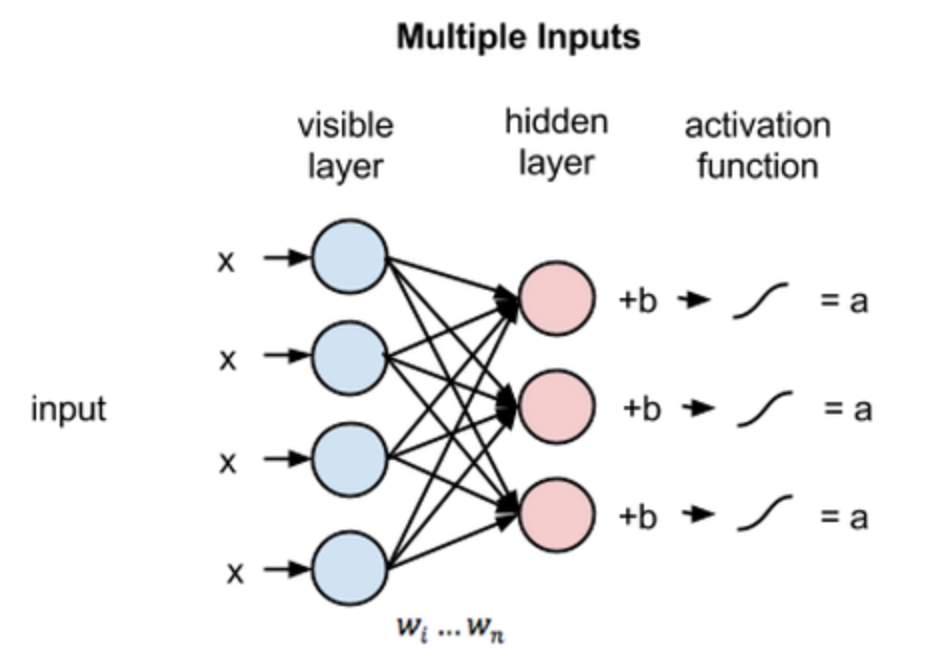
As the image above shows, each hidden node receives input from all nodes from the visible layer (4 in this case), multiplied by their respective weights. The result is then added to a bias (which at least forces some activation to occur), followed by the activation algorithm, producing one output for each node.

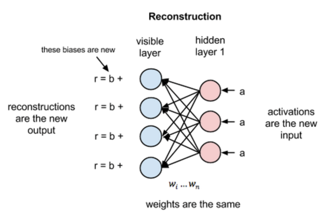
During the reconstruction phase, the activations of the hidden layer become the input in a backward pass. They are multiplied by the same weights, and are then added to another bias (the visible layer bias) and the output is considered a reconstruction. Therefore, the reconstruction error is the error between the reconstruction (r in the image) and the original input. The error is backpropagated against the weights in an iterative learning process until a minimum error is reached.

Formatting data for RBM input
A dataframe cannot be fed into the RBM model in TensorFlow. We will have to turn it into a list of lists. The list will have 1490 lists within, which represents each user. For each user’s list, there will be 1186 values, which corresponds to the number of items (books). The values are the user’s ratings, and it is a zero if the user did not rate the item.

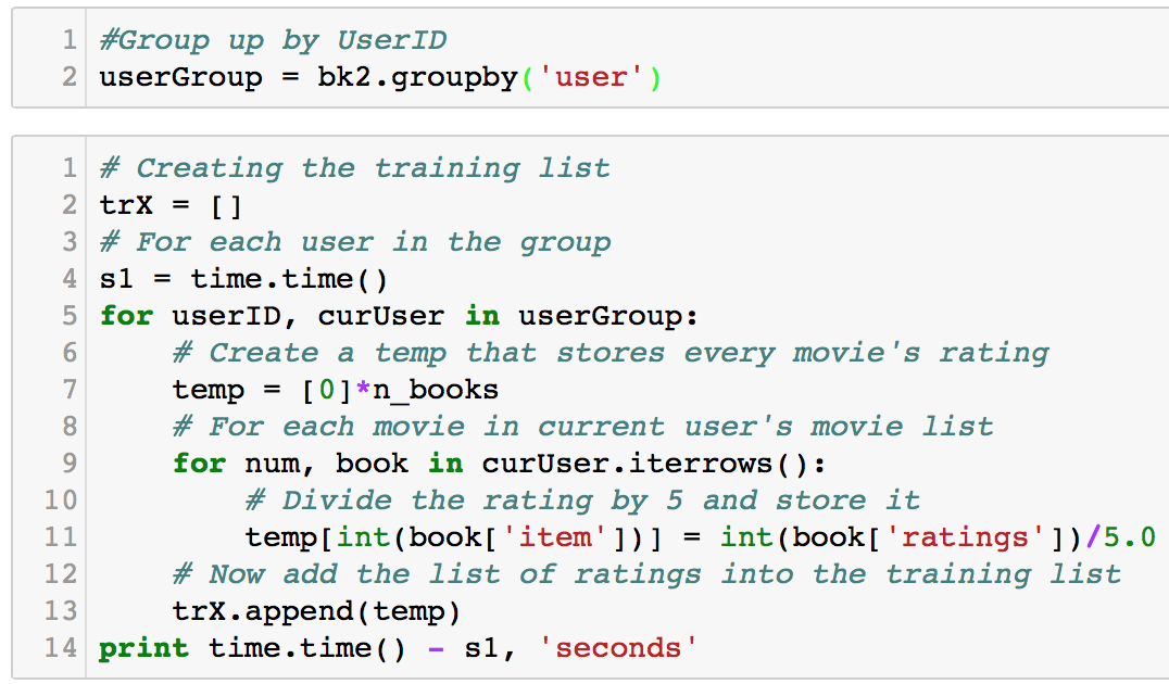
First, we use pandas’ groupby to group the dataframe by users. Then, we iterate and append rating values to a temporary list, which then gets appended to the main list (trX).

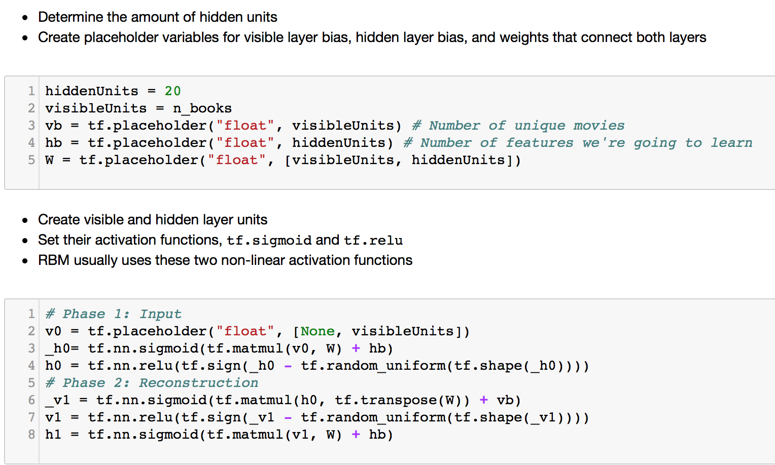
We begin by creating the layers, both visible and hidden. In the code, the biases are created first. The number of nodes in the hidden layer can be chosen and set, whereas the visible layer will have number of nodes equal to the number of unique items in our data. This is because each of our input data is a list of all ratings for all items of one user.
Next, we create the Weights layer which will be multiplied with the visible layer and fed into the hidden layer. That is why it has the shape with rows = number of visible nodes, and columns = number of hidden nodes.
The second box is where we create the layers, input and reconstruction. We use a sigmoid activation function because we have formatted the input to be continuous between 0 and 1. Next, we use tf.sign on the hidden layer and have a ReLU function act on it. The reconstruction phase is just a reverse of the above.

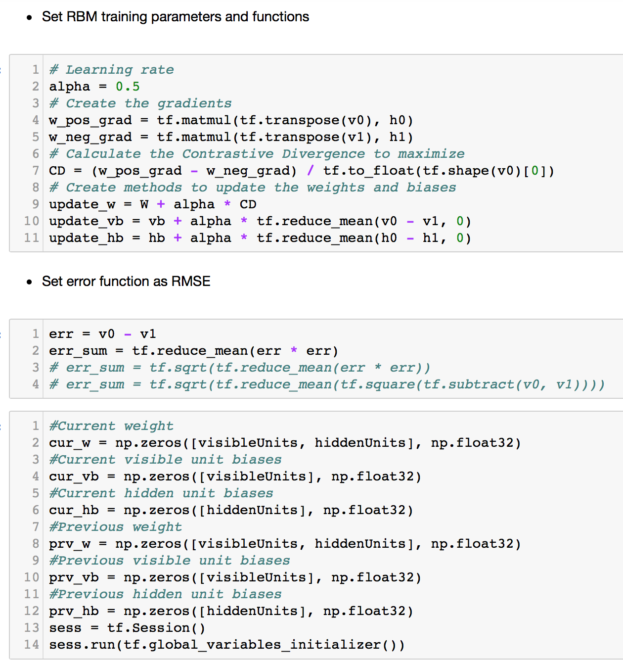
First, we set our equations for Contrastive Divergence to update the weights. A learning rate is also set. Next, the updating of Weights and Biases are carried out.
The error function is then defined. It is simple the mean squared error of the output minus the input. This gives us the reconstruction error which tells us how different the output is from the input. We are aiming to reduce this MSE as we want the machine to learn to reconstruct the input, and come up with weights and biases that allow for this. Lastly, we create the values for the placeholders. Finally, we run the model with the code below!

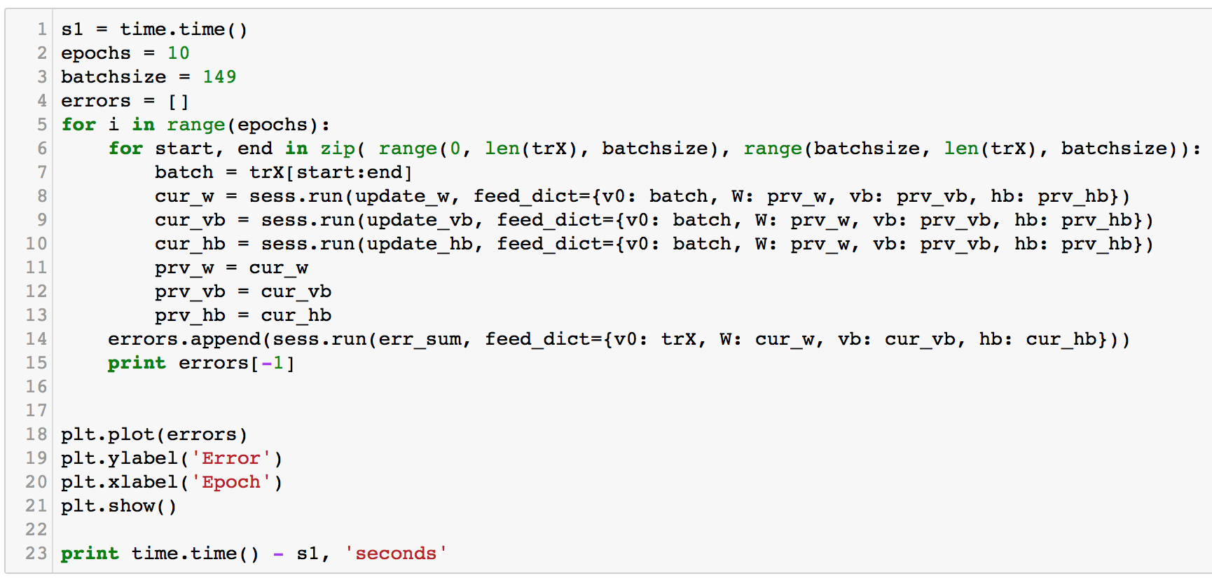
The first and last lines of time.time() shows us how long the entire training took. Each epoch refers to a full training where the entire dataset is used. In this example, we will train the entire dataset 10 times. The ‘update’ equations are run to update the current weights and biases, and thereafter they will be assigned as ‘previous’, which will then be fed into the new epoch. We only specify to run the ‘update’ because everything that is linked (before) to the ‘update’ equation will also be run. These iterations continue to update the weights and biases while reducing the reconstruction error.

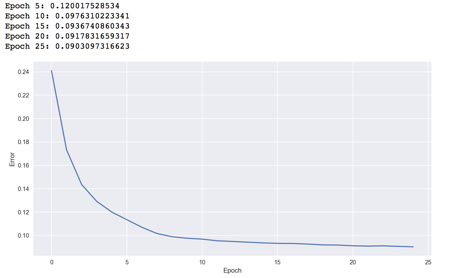
The figure only shows the reconstruction error of the first 25 epochs. The error reduces rather quickly and slows down after 0.09. Thereafter, the training ran and completed 1000 epochs which further reduced the error to about 0.81 where it seemed to stagnate (view in Jupyter Notebook).

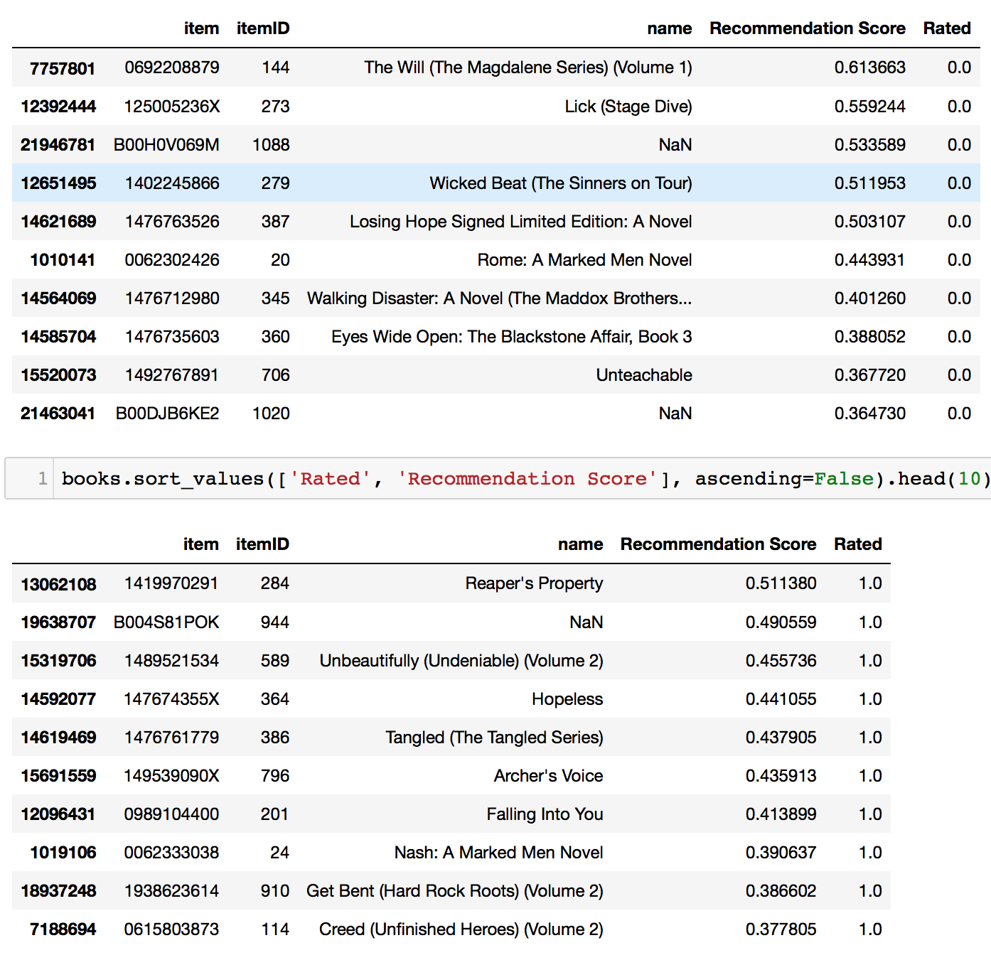
Now that our training has reached stability, we check its performance by generating recommendations. The first table above shows the machine’s recommendations, and the second table shows the user’s rated books. For both tables, we can see the predicted ratings of our machine from the column “Recommendation Score”.

Please feel free to look up these books to find out what they are! I have done so and discovered that the user rated highly books about Romance. The books that our model recommended belonged to Romance as well, which also coincides with our matrix factorisation model. That’s good to know.

Evaluation

Thus far, we ran 3 models which gave us fairly similar results.

• Matrix Factorisation optimised by ALS/SGD
• Multiple Surprise package models
• Restricted Boltzmann Machine

Future Work

I'm excited to try Content Based methods, which include Approximate Nearest Neighbours, definitely Wide and Deep networks.

Moving on, I would want to try Deep Matrix Factorisation using TensorFlow and/or Apache MXNet. Recent attempts have shown that deep learning allows to learn more sophisticated models which can take in more complicated inputs (as compared to traditional matrix factorisation), potentially yielding additional insight into the task. As Andrew Ng mentioned, A.I. is the new electricity. Therefore, more work will go into exploring RecSys through deep learning. On a different note, Graph solutions like neo4j is worth exploring too.